This book makes a great reference manual for using GDAL/OGR suite of command line …,
January 24, 2015 By Leo Hsu
“The GDAL Toolkit is chuckful of ETL commandline tools for working with 100s of spatial (and not so spatial data sources). Sadly the GDAL website only provides the basic API command switches with very few examples to get a user going with. I was really excited when this book was announced and purchased as soon as it came out. This book makes a great reference manual for using GDAL/OGR suite of command line utilities.
Several chapters are devoted to each commandline tool, explaining what its for, the switches it has, and several examples of how to use each one. You’ll learn how to work with both vector/(basic data no vector) data sources and how to convert from one vector format to another. You’ll also learn how to work with raster data and how to transform from one raster data source to another as well as various operations you can perform on these.”
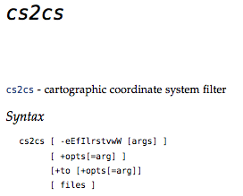
If you have files or apps that have to filter or convert coordinates – then the cs2cs command is for you. It comes with most distributions of the GDAL/OGR (gdal.org) toolset. Here is one popular example for converting between degrees minutes and seconds (DMS) and decimal degrees (DD).
Input coordinates can come from the command line or an external file. Assuming a file containing DMS (degree, minute, seconds) style, looks like:
124d10'20"W 52d14'22"N

122d20'05"W 54d12'00"N
Use the cs2cs command, specifying how the print format will be returned, using the -f option. In this case -f “%.6f”
is explicitly requesting a decimal degree number with 6 decimals:
Geospatial Power Tools is 350+ pages long – 100 of those pages cover these kinds of workflow topic examples. Each copy includes a complete (edited!) set of the GDAL/OGR command line documentation as well as the following topics/examples:
Geospatial Power Tools by Tyler Mitchell now on Amazon
Ten years ago I wrote a book for O’Reilly called Web Mapping Illustrated – using open source GIS tools. It was mostly about how to use MapServer and PostGIS to publish maps on the web and was the first of its kind in the marketplace.
This year I’ve completed my second book, for Locate Press, which focused on even more low level geospatial data manipulation using the GDAL/OGR command line tools. This was a work-in-progress for a couple of years, but has just now been released on Amazon as Geospatial Power Tools.
If you’re looking for a resource to understand how to convert imagery, vector data or to build elevation shaded maps or contours, and more, then this book is for you. It includes complete GDAL and OGR documentation. A third of the book presents new material geared to help you learn how to do specific kinds of processing tasks – from downloading from web services, to quickly converting imagery into an online map. A PDF version is also available and Kindle will likely come over the next 6 months.
I’m always interested in feedback on the book and to learn more about how to improve the next edition.
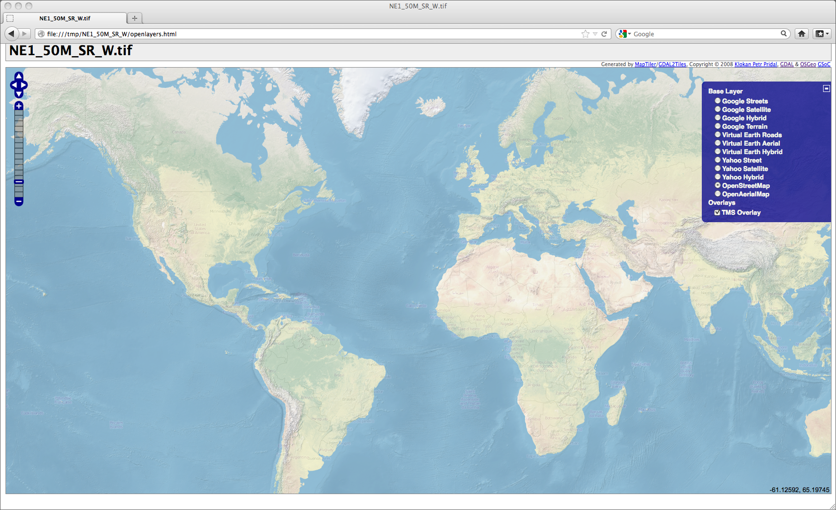
Tiles in a Tile Map Server (TMS) context are basically raster map data that’s broken into tiny pre-rendered tiles for maximum web client loading efficiency. GDAL, with Python, can chop up your input raster into the folder/file name and numbering structures that TMS compliant clients expect.
Default OpenLayers application produced by the gdal2tiles command and a Natural Earth background dataset as input.
This is an excerpt from the book: Geospatial Power Tools – Open Source GDAL/OGR Command Line Tools by me, Tyler Mitchell. The book is a comprehensive manual as well as a guide to typical data processing workflows, such as the following short sample…
The bonus with this utility is that it also creates a basic web mapping application that you can start using right away.
The script is designed to use georeferenced rasters, however, any raster should also work with the right options. The (georeferenced) Natural Earth raster dataset is used in the first examples, with a non-georeferenced raster at the end.
There are many options to tweak the output and setup of the map services; see the complete gdal2tiles chapter for more information.
Open the openlayers.html file in a web browser to see the results.
The default map loads a Google Maps layer, it will complain that you do not have an appropriate API key setup in the file, ignore it and switch to the OpenStreetMap layer in the right hand layer listing.
The resulting map should show your nicely coloured world map image from the Natural Earth dataset. The TMS Overlay option will show in the layer listing, so you can toggle it on/off to see that it truly is loading. Figure 5.2 (above) shows the result of our gdal2tiles command.
Geospatial Power Tools is 350+ pages long – 100 of those pages cover these kinds of workflow topic examples. Each copy includes a complete (edited!) set of the GDAL/OGR command line documentation as well as the following topics/examples:
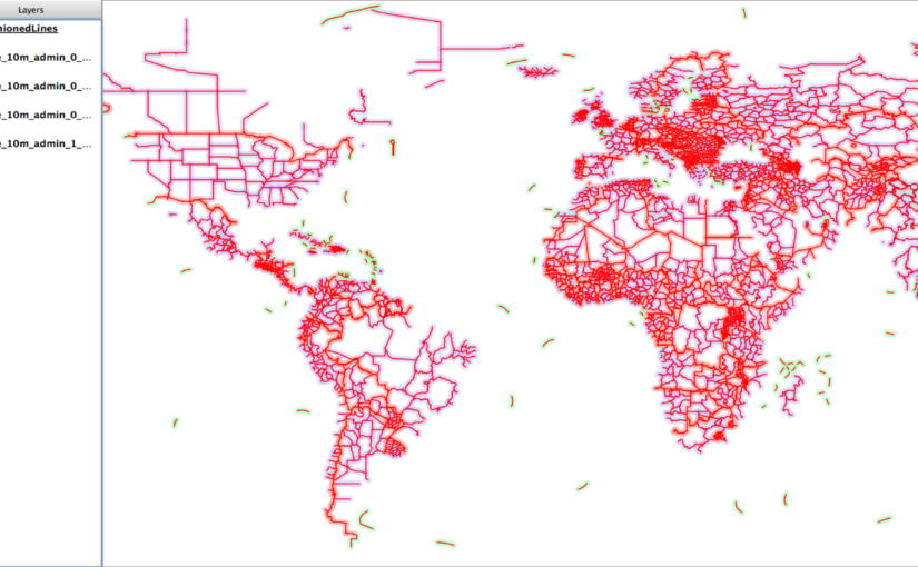
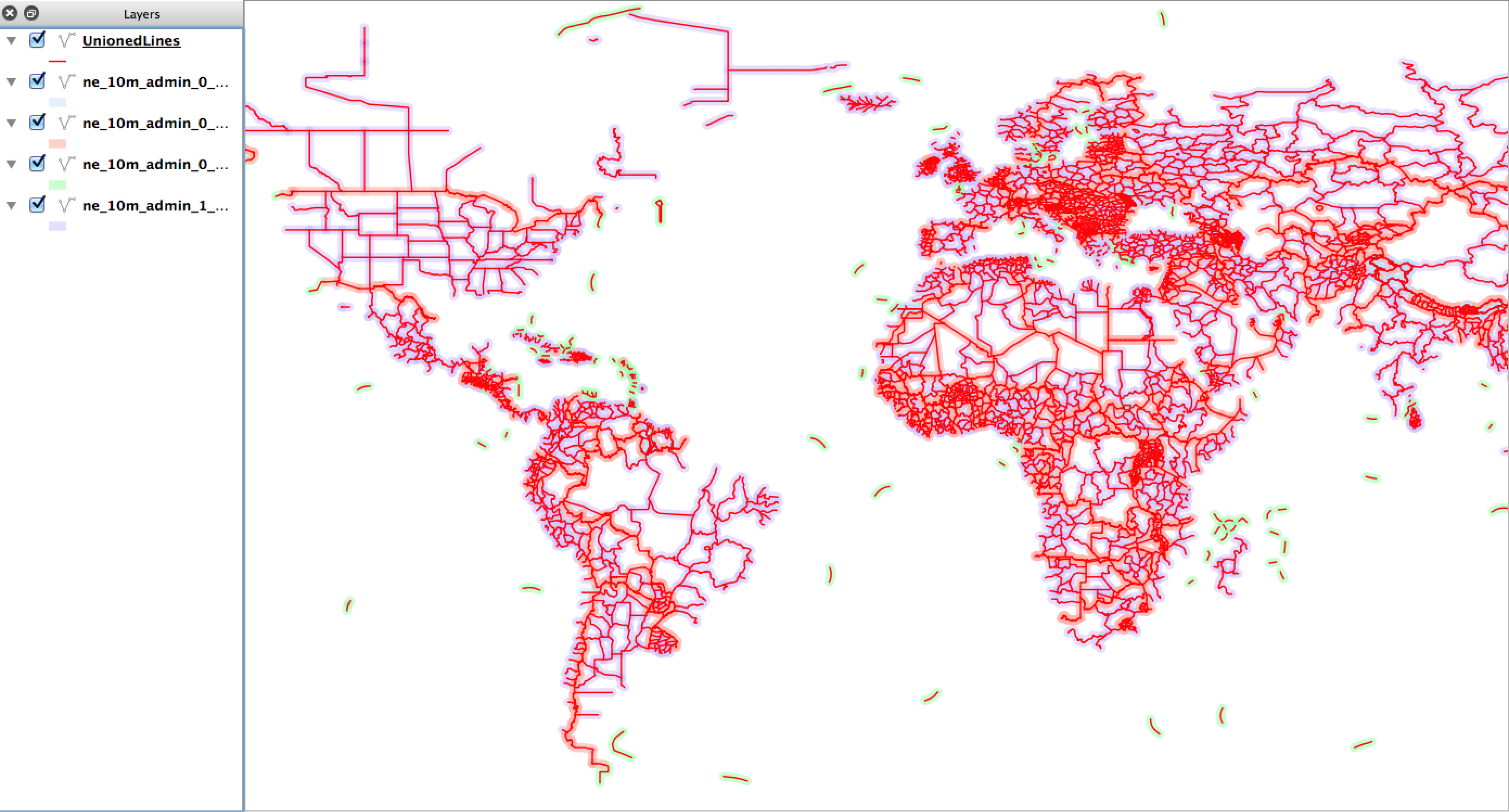
The real power of VRT files comes into play when you want create virtual representations of features as well. In this case, you can virtually tile together many individual layers as one. At the present time you cannot do this with a single command line but it only takes adding two simple lines to the VRT XML file to make it start working.
Here we want to create a virtual vector layer from all the files containing lines in the ne/10m_cultural folder.
First, to keep it simple, create a folder and copy in only the files we are interested in:
If added to QGIS at this point, it will merely present a list of four layers to select to load. This is not what we want.
So next we edit the resulting all_lines.vrt file and add a line that tells GDAL/OGR that the contents are to be presented as a unioned layer with a given name (i.e. “UnionedLines”).
The added line is the second one below, along with the closing line second from the end:
Now loading it into QGIS automatically loads it as a single layer but, behind the scenes, it is a virtual representation of all four source layers.
On the map in Figure 5.8 the unionedLines layer is drawn on top using red lines, whereas all the source files (that I manually loaded) are shown with a light shading. This shows that the new virtual layer covers all the source layer features.
Geospatial Power Tools is 350 pages long – 100 of those pages cover these kinds of workflow topic examples. Each copy includes a complete (edited!) set of the GDAL/OGR command line documentation as well as the following topics/examples:
Use a SQL-style -where clause option to return only the features that meet the expression. In this case, only return the populated places features that meet the criteria of having NAME = ’Shanghai’:
Building on the above, you can also query across all available layers, using the -al option and removing the specific layer name. Keep the same -where syntax and it will try to use it on each layer. In cases where a layer does not have the specific attribute, it will tell you, but will continue to process the other layers:
ERROR 1: 'NAME' not recognised as an available field.
NOTE: More recent versions of ogrinfo appear to not support this and will likely give FAILURE messages instead.
Geospatial Power Tools is 350 pages long – 100 of those pages cover these kinds of workflow topic examples. Each copy includes a complete (edited!) set of the GDAL/OGR command line documentation as well as the following topics/examples:
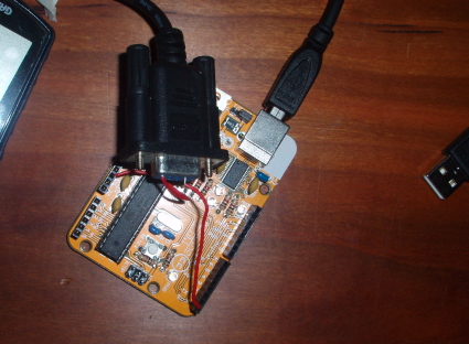
With OSSIMPlanet’s nifty camera control and listener functionality, as demonstrated in my last post, you’ve got so many neat opportunities. A couple nights ago I got a basic GPS NMEA parser working. Here’s a pic of the ultra-professional connection method I use to hook it to my arduino board 🙂
Two wires to hook an eTrex data cable up to the Arduino
Oops, just realised that the picture shows the wires in the wrong spot (it was a late night photo). Pin 2 from the serial cable goes into the Power GND on left side of board. Pin 5 from serial cable goes into the Digital Pin 0 aka RX pin on lower right.
Note that I had a lot of confusion regarding the pin-out options for the Etrex. I looked at several diagrams and couldn’t get the right pins to work. It appears that you may actually need to swap the ground/TX pins to make it work – that’s what I had to do. This is something to do with how the serial connection works.. something I won’t pretend to understand – but swapping the wires worked, that’s all I know!
Of course you could always use your nifty new bluetooth GPS receiver, or plug your receiver directly into the PC and this would still work. But for me, I will have additional devices going into the arduino, where their signals will get mixed together before being sent to the PC.
Arduino setup
The arduino doesn’t do much here, except filter the strings coming from the GPS. It grabs only the $GPGGA string that has the location info I want. I specifically used the GPGGA because the Python NME parser code example I had used that one and I didn’t want to have to learn how to handle the $GPRMC strings.
Here’s the basic code I run on the Arduino:
Tmitchell: on etrex port - pin 1 (at notch end) is for TX and pin 3 for GND
On serial cable out Pin 2 -> GND, Pin 5 as TX (hooks to Digital 0=RX on board)
*/
#include <string.h>

#include <ctype.h>
int ledPin = 13;                  // LED test pin
int rxPin = 0;                    // RX PIN
int txPin = 1;                    // TX TX
int byteGPS=-1;
char linea[70] = "";
char comandoGPR[7] = "$GPGGA";
char latdms[9], londms[10], latdir[1], londir[1] = "";
int latdd, londd, heading = 0;
int cont=0;
int bien=0;
int conta=0;
int indices[13];

void setup() {
  pinMode(ledPin, OUTPUT);       // Initialize LED pin
  pinMode(rxPin, INPUT);
  pinMode(txPin, OUTPUT);
  Serial.begin(4800);
  for (int i=0;i<70;i++){       // Initialize a buffer for received data
    linea[i]=' ';
  }
}
void loop() {
  digitalWrite(ledPin, HIGH);
  byteGPS=Serial.read();         // Read a byte of the serial port
  if (byteGPS == -1) {           // See if the port is empty yet
    delay(100);
  } else {
    linea[conta]=byteGPS;        // If there is serial port data, it is put in the buffer
    conta++;
    if (byteGPS==13){            // If the received byte is = to 13, end of transmission
      digitalWrite(ledPin, LOW);
      cont=0;
      bien=0;
      for (int i=1;i<7;i++){     // Verifies if the received command starts with $GPR
        if (linea[i]==comandoGPR[i-1]){
          bien++;
        }
      }
      if(bien==6){               // If yes, continue and process the data
        for (int i=0;i<70;i++){
          if (linea[i]==','){    // check for the position of the  "," separator
            indices[cont]=i;
            cont++;
          }
          if (linea[i]=='*'){    // ... and the "*"
            indices[12]=i;
            cont++;
          }
        }
          Serial.print(linea);  // This is the important line :)
      }
      conta=0;                    // Reset the buffer
      for (int i=0;i<70;i++){    //
        linea[i]=' ';
      }
    }
  }
}
I had originally hoped to do the XML prep in the arduino, but skipped it for now due to my poor understanding of variable types in the processing language. So for now I’ve still got a lot of cruft leftover in the above, that I didn’t need from the original tutorial code. But as I add more sensors I’ll want to do more mixing in the board itself.
So the arduino board just sends a raw NMEA $GPGGA string to the serial port, where Python takes over.
Python Serial Reader and OSSIM Controller
I then use a Python script that checks for strings coming from the arduino board. It does a bit of filtering, but not much error checking at the moment. This is the first time I’ve used Python to connect to the serial port, so it was fun to learn and so simple!
I found this GPGGA parser code and incorporated it into my script. I won’t paste it here as it is quite long. But here is the rest of my script – reading from Serial, parsing results, then reformatting and sending to OSSIMPlanet… comments, cruft and crummy coding.. all yours for free!
Be sure to have OSSIMPlanet running and set its Preferences to listen on port 5000 first.
# Uses PySerial
import serial

# GPGGA Parsing code next

class GPGGAParser(object):
import logging

# Open connection to Arduino
s = serial.Serial('/dev/cu.usbserial-A6001VQr', 4800, timeout=1) heading = 0
# initialising here so I can rotate the heading during each cycle.. just for fun

# Read Arduino output

while (1>0):
char = s.read(1)
while (char <> '$'):
char = s.read(1)
else:
sentence = '$' + s.read(70)
# Parse output
#############
print sentence.strip()
if (len(sentence.strip())<=30) or (sentence[1:5] <> 'GPGG'):
continue
else:
parsed = GPGGAParser(sentence)

if (parsed.latitude <> 0 and parsed.longitude <> 0):

#####################
# Reformat to XML
## Hacked method first
heading += 10 # during testing I never moved,
# so I made it hover over my location and
# slowly spin 10 degrees each second
if (heading >= 360): heading = heading-360
pitch = 70
altitude_mult = 10
ossimxml = '<Set target=":navigator" vref="wgs84"><Camera><longitude>%s</longitude><latitude>%s</latitude><altitude>%s</altitude><heading>%s</heading><pitch>%s</pitch><roll>0</roll><altitudeMode>absolute</altitudeMode></Camera></Set>' % (parsed.longitude, parsed.latitude, parsed.altitude * altitude_mult, heading, pitch)
print ossimxml # show xml being sent to ossimplanet
## Proper DOM tools second - will do this "right" at some point :)
## But not written yet

#######
# Open connection to OSSIMPlanet listener
import socket
ossim = socket.socket(socket.AF_INET, socket.SOCK_STREAM)
ossim.connect(("127.0.0.1", 5000))
# Send view updates
# Optional: connect to OSSIMPlanet broadcaster
## adjust coordinates based on current view
## I will do this when using nunchuks, but for now nothing
ossim.send(ossimxml)
ossim.close()
# Lather, rinse, repeat....
That’s about it. In OSSIMPlanet the updates are practically instantaneous, but I wait 1 sec for new GPS data to come in. When I start using the nunchuks I’ll want to do more updates faster to emulate the movement smoother. But that’s for another day…