This past year I started using GeoServer more than I did before. Actian is using it to demonstrate the capabilities of the Ingres 10S database sitting behind it. So I was glad to see that there was a new book out on the topic, by Stefano Iacovella and Brian Youngblood.
It was very readable and went faster than I thought it would (maybe it would have been longer if I didn’t skip a few exercises 😉 ). The book opens with the standard GIS Fundamentals but by the end of it you can be hacking XML and hitting the REST interface.
A few highlights to consider… Those who struggle with getting started with Tomcat on Linux will appreciate the chapter on installation. Likewise there is a chapter pointing out how to better secure everything before going into production.
The book is packed full of screenshots and graphics, making it very easy to follow along. The authors also did a great job making it readable and accessible. I would recommend it for anyone who is a first time GeoServer user. Check it out here.
When innovation is sought after, for example in the government open data initiatives, it becomes even more important to have effective connection with people in the trenches.
I propose the use of collaborative meeting spaces, a sort of Demilitarized Zone for government and constituents to connect – physical places where they can meet together, and not just so they can meet face-to-face, but to implement an innovative (new?) way of making spontaneous collaboration happen…
Those who know me are likely sick of my retelling of stories about my observations on the impact of migrating away from command line GIS (circa ArcInfo Workstation) to the typical desktop GIS with graphical user interfaces. More often than not, however, my desire for server-side scripting is now done within spatial databases (Ingres and Postgres/PostGIS databases being the two I recommend the most). The interface between the GIS client and the server is still ripe for innovation however.
While some desktop applications can leverage server-side processes, instead of pulling it all down to the client, I have seen it less in-the-wild than I have the traditional client-side approach. I’m hopeful that with products like ArcGIS Server, GeoServer or even GIS Cloud, PyWPS, deegree, 52North, Zoo, etc. much of that work will finally be put where it belongs.
Enter the Web Processing Service (WPS) to help glue it all together. A couple years back I barely knew this existed, but now that it is easy to enable this on GeoServer, it’s starting to draw my attention more and more. However, I can’t help but think that lack of client support is hampering the adoption of a WPS-based workflow. When I saw there was a WPS plugin for QGIS then I really started paying attention!
Here’s why…
Imagine having layers loaded, say, through a WFS. So you’re just drawing some features, selecting a few and then sending off a request to the server to process a buffer or to do a clip function. Behind the scenes, QGIS would send just the select shape of interest, tell the server what process to run (along with some other parameters) and return the result to your map view. Only a few local temporary files and all is done in one spot and kept clean.
Too good to be true? You be the judge and let me know 🙂
p.s. The ultimate end game for me here is to have my Ingres spatial db serving up customer data via WFS, with options to process the data with GeoServer WPS. I’ve tested against other platforms with more success, but I’ve only gotten halfway there with GeoServer. If you’ve done QGIS with WPS plugin against a GeoServer WPS instance, I’d like to hear from you (twitter: spatialguru). I can get it to create a grid, for example, but I can’t get the client to send data to the server and get a result.
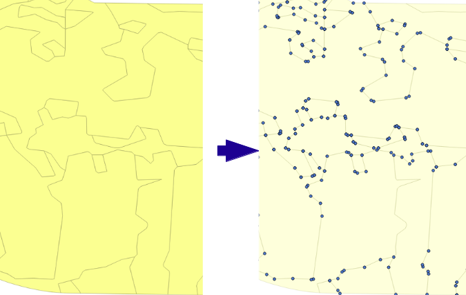
How do I convert my linestring shapefile into points?
It’s a common enough question on the OSGeo mailing lists and stackexchange.com. Even with the power of GDAL/OGR command line utilities, there isn’t a single command you can run to do a conversion from lines/polygons into points. Enter ogr_explode.py.
I’ve co-opted the term “explode” to refer to this need and put together a simple Python script to show how it can be done. You can access it on GitHub here or see just the main guts of it listed below.
It’s just a start, without any real error checking, and can be greatly improved with more options – e.g. to take elevation from the parent lines/polys attributes, to output to another shapefile, etc. Because it outputs in a CSV (x,y,z) format, you can give it a .csv extension and start to access it with OGR utilities right away (VRT may be required). For example, you could then push it through gdal_grid, but that’s another topic…
Since it is a common enough need, it seems, I encourage you to fork a copy and share back.
[Note, QGIS has a nice option under its Vector -> Geometry Tools -> Extract Nodes tool to do the same thing with a GUI. Props to NathanW for having the most easily accessible example to refer to 🙂 ]
...

for feat in lay:

geom = feat.GetGeometryRef()

for ring in geom:

points = ring.GetPointCount()

for p in xrange(points):

lon, lat, z = ring.GetPoint(p)

outstr = "%s,%s,%s\n" % (lon,lat,z)

outfile.write(outstr)

...
From Locate Press: “We don’t have a cover to tease you with, but we have started a website where you can learn more: http://pythongisbook.com · The PyQGIS Programmers Guide. Extending Quantum GIS with Python. This all ne…Read more…“
As in my previous post, you can see how a generic approach to taking irregularly spaced text format data may be applied to a wide range of contexts. In this post I show a particular example of taking some freely available LIDAR result data and processing it with the same approach.
Get the Data
To follow along, you can grab the same data I did from OpenTopography.org. You can find your way through their search tools for an area of interest.
Unzipping the file produces a 138MB text file called points.txt. This is already in a format that OGR can read, but to help it along just rename the file to points.csv and we don’t have to mess around changing the delimiter (as in previous post). Note the first line contains column headings too, so this is a perfect example to be using:
In case it wasn’t clear previously, we create a VRT file so that gdal_grid (or any OGR application) knows how to find the X/Y coordinates in the CSV file. So we just create and tweak like in the previous example but include the field names that are already in points.txt, etc. Here is our new points.vrt file:
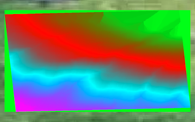
Here’s the part that takes a while. With > 2 million rows it takes a bit of time to process, depending on what algorithm settings you use. To just use the default (inverse distance to a power) run it without an algorithm option:
gdal_grid -zfield z -l points points.vrt points.tif


Grid data type is "Float64"

Grid size = (256 256).

Corner coordinates = (329998.848164 7002001.415547)-(330590.891836 7001268.684453).

Grid cell size = (2.303672 2.851094).

Source point count = 2267774.

Algorithm name: "invdist".

Options are "power=2.000000:smoothing=0.000000:radius1=0.000000:

radius2=0.000000:angle=0.000000:max_points=0:min_points=0:nodata=0.000000"
I also got good results from the using the nearest neighbour options as shown in the gdal_grid docs. Note it creates a 256×256 raster by default. In the second example it shows how to set the output size (-outsize 512 512). The second example took about an hour to process on my one triple core AMD 64 desktop machine with 8GB RAM:
gdal_grid -zfield z -outsize 512 512 \

-a nearest:radius1=0.0:radius2=0.0:angle=0.0:nodata=0.0 \

-l points points.vrt points_nearest_lrg.tif


Grid data type is "Float64"

Grid size = (512 512).

Corner coordinates = (329999.424082 7002000.702773)-(330590.315918 7001269.397227).

Grid cell size = (1.151836 1.425547).

Source point count = 2267774.

Algorithm name: "nearest".

Options are "radius1=0.000000:radius2=0.000000:angle=0.000000:nodata=0.000000"
A common question that seems to come up on the GDAL discussion lists seems to be:
How do I take a file of text data or OGR readable point data and turn it into an interpolated regular grid?
Depending on what your source data looks like, you can deal with this through a three step process, but is fairly straightforward if you use the right tools. Here we stick to just using GDAL/OGR command line tools.
1. Convert XYZ data into CSV text
If the source data is in a grid text format with rows and columns, then convert it to the XYZ output format with gdal_translate: gdal_translate -of XYZ input.txt grid.xyz
If your source data is already in an XYZ format, or after above conversion, then change the space delimiters to commas (tabs and semicolon also supported). This is easily done on the command line using a tool like sed or manually in a text editor:
sed 's/ /,/g' grid.xyz > grid.csv
The results would look something like:
-120.5,101.5,100

-117.5,101.5,100

-116.5,100.5,150

-120.5,97.5,200

-119.5,100.5,100
2. Create a virtual format header file
Step 3 will require access to the CSV grid data in an OGR supported format, so we create a simple XML text file that can then be referred to as a vector datasource with any OGR tools.
Create the file grid.vrt with the following content, note the pointers to the source CSV file and the fields which are automatically discerned from the CSV file on-the-fly:
<OGRVRTDataSource>

<OGRVRTLayer name="grid">

<SrcDataSource>grid.csv</SrcDataSource>

<GeometryType>wkbPoint</GeometryType>

<LayerSRS>WGS84</LayerSRS>

<GeometryField separator=" " encoding="PointFromColumns" x="field_1" y="field_2" z="field_3"/>

</OGRVRTLayer>

</OGRVRTDataSource>
If the first row of the grid.csv file includes custom field names, e.g. X, Y, Z, then substitute them for the field_1, field_2 and field_3 settings above.
3. Convert using gdal_grid
Now for the following step, convert this OGR vector VRT and CSV format into a GDAL raster format, while also interpolating any “missing” points in the grid. Various options are available for interpolating. See gdal_grid command syntax for more information, a minimal example is shown here using all the defaults:
gdal_grid -zfield field_3 -l grid grid.vrt newgrid.tif
The output product will fill in any holes in the source grid. Several algorithms are available, the default uses the inverse distance to a power option.
Those of us involved with open source geospatial software already know that you must innovate or die. Okay, maybe that’s a bit dramatic, but I know many of us feel like we will die if we do not continually learn more and be challenged. I just wrote an article that tries to articulate some of the areas where we need to keep our muscle stretched. This is especially for those who are looking at their career in horror – wondering when their skills will be leap-frogged into oblivion by a recent grad who happened to spend more time learning on his/her own time.
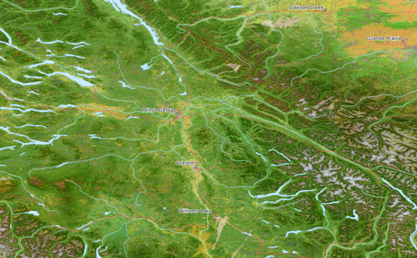
Following from my last post, if you’re looking for a site for “framework” Canadian geodata, check out GeoBase.ca, including layers such as: hydrographic, road network, various admin boundaries, imagery, and more.. all for free download.
But today I’m pulling it in using their WMS option to dynamically view the data without downloading:
I hope we’ll see more provinces get in on the action and start putting more higher res imagery up for WMS feeds, but for now I’m not complaining. Keep up the good work! If you enjoy it too, let them know by encouraging them with good feedback.
By the way, anyone know of an Ontario higher res imagery WMS or download site?
 It was very readable and went faster than I thought it would (maybe it would have been longer if I didn’t skip a few exercises 😉 ). The book opens with the standard GIS Fundamentals but by the end of it you can be hacking XML and hitting the REST interface.