Tag: graph

I’ve been spending a lot of time this past year running queries against the open source SPARQLverse graph analytic engine.  It’s amazing how simple some queries can look and yet how much work is being done behind the scenes.

My current project requires building up a set of query examples that allow typical kinds of graph/network analytics – starting with the kinds of queries needed for Social Network Analysis (SNA), i.e. find friends of friends, graph density and more.

In this post I go through computing graph density in detail.

First of all I’d love to hear what your favourite SPARQL query patterns are in this space.  Please ping/tweet me if you have some that you find yourself using over and over!

My starting point is with some of the samples SPARQLcity makes available on their tips and tricks page.  Let’s first look at a sample dataset and then apply a couple of these to a query problem.

Installing SPARQLverse Graph Analytic Engine

Installing SPARQLverse on a Linux machine is dead simple (you’ll need 8GB RAM by default):

1. Download latest (binary) release (open source code is available as well!)
2. Unzip the file
3. Launch the startup script:

   1. rel/bin/sbxstart

4. Use web console at http://localhost:8080
5. Now if you have an RDF/Turtle format triples file you can load it via command line – provide the name of graph to create, and your input filename:

   1. ploadsbx mygraph graph_friends.ttl
      

Sample Turtle Format Data for SPARQL

Don’t be scared away from RDF/Turtle or triple stores in general due to the new format.  Triples don’t get much simpler than just three URIs or even just three distinct words on a line.

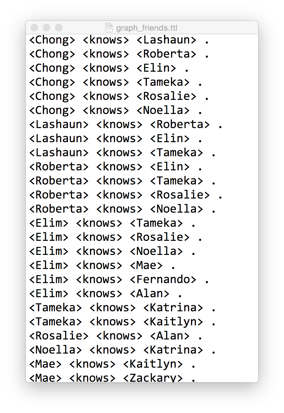
Here is what a sample looks like (graph_friends.ttl) that we can load into SPARQLverse with the above command:

It includes 57 specific relationships. The first part of the triple is the Subject, the second is the Predicate/relationship made to the third part, the Object. If you look through the data you’ll see that all the Objects are also defined as Subjects that have other relationships.

Understand the basics here and you’ve got Triples almost mastered.

Note: This is an overly simplistic example, but not totally unrealistic.  We don’t use any URIs but we are allowed to fake them here by simply putting angle brackets around them.  In a linked data environment you’d establish your own namespaces and likely link to external SPARQL endpoints or resources with http:// prefixes.  Now that starts to make your eyes crossed.

Quick Visualisation

As an aside, pull the sample data into Gephi to visualise it and you’ll see the intertwining relationships are not intuitive and would be a challenge to understand using a SQL relational approach.

What is the Density of the Social Network?

Back to the SPARQL tips page…

What is Graph Density?

Graph density represents how interconnected all entities in the graph are.  They are  a sort of ratio between the total number of connected nodes over maximum number of potential edges.  The value ranges from 0 to 1 – with 0 being a total disconnected graph (not sure if that is technically a graph) with no interconnections between nodes.  And 1 representing a high density graph where all nodes connect to all other nodes.

Here we use a SPARQL query to compute graph density, using the sample dataset above, run from the command line. (Note that I use “?knows” as a predicate when I really want to use “<knows>” but wordpress is not displaying that properly):

$ isbx -c "
 SELECT (?nrEdges/(?nrNodes *(?nrNodes - 1.0)) AS ?graphDensity)
 FROM <graphname>
 WHERE {
  { SELECT (COUNT (*) AS ?nrEdges) (COUNT (DISTINCT ?person) AS ?nrNodes)
    WHERE { ?person ?knows ?anotherPerson . }
   }
 }
"
graphDensity
-------------
0.150000

I changed the example “tips” query to use a different graph name (mygraph) and a different relationship name (knows).  The sub-query in the WHERE clause first counts up the number of edges/relationships and counts the distinct number of nodes as well.  Then the primary query compares that number of edges to nodes.

Let’s break that down into its detail…

Compute the number of unique nodes in the graph

$ isbx -c "SELECT (count (distinct ?person) as ?nrNodes)
> FROM <graphname> WHERE { ?person ?knows ?anotherPerson .}"
nrNodes
--------
20

This tells us that there are 20 people as Subjects in the graph.  Therefore, a maximum number of edges between all people would be 20² (we’ll use only 20×19 as a person might not link to themselves in this example).

Compute the number of edges in the graph

$ isbx -c "SELECT (count (*) as ?nrEdges)
FROM <graphname> WHERE { ?person ?knows ?anotherPerson .}"
nrEdges
--------
57

Total edges is 57.  Do the quick math and see that the ratio is then:

57 / (20 x 19)
= 57 / 380
= 0.149...

Challenge: Inverse Relationships in SPARQL

In some graphs you may not have all the people in the Object position (third part of triple) initialised as Subjects – and their names only show up when someone else defines a relationship to them.

In that case, your density from this query will under-report.  I leave it as an exercise to the reader to figure out how to use SPARQL to do an optional inverse relationship in the sub-query WHERE clause.  Ping me if you want some tips on that.

Future Post

In a future post I’ll walk through some of other graph query examples using SPARQL such as:

• Who has the most friends who know each other?
• What is the size of a person’s network?

What else is important to you?  Let me know!

SPARQLverse is part of the Actian Analytics Platform – providing Big Data solutions that are hyper performance with ultimate scalability. Our SQL in Hadoop is the fastest available and runs truly in Hadoop 100%.