Kibana dashboards, from the Elasticsearch project, can help you visualise activity and incidents in log files. Here I show 3 different types of use cases for dashboards and how each can be used to answer different questions depending on the person. Video and details follow.
The first example is the simplest UI I could imagine: a query/search box, a histogram, and a table. In this instance any user, at any level of curiosity, can find textual data in the logs using a keyword match.
Then they can also see the relative number of records that occur at given times within the time window of all the data available. These are aggregate counts of all records that have some match to the query keyword or algebra.
Likewise, the table reflects the subset of data provided by the records, with the ability to only show fields of interest.
Process Details
A slightly more advanced use is to focus on a particular process (i.e. application) running on a machine that’s being logged. Here we can then take a particular metric, i.e. CPU usage, and graph it instead of just a simple histogram.
A typical user may be in charge of a particular set of services in a system. Here they can see how they perform and yet still dig into the details as desired.
I also do some cool “markers” to subtly show when events coincide with other process metrics.
All Events
The data example shown here has process, performance and event logging information. I combine multiple queries and having them drive different parts of the dashboard – a pie chart, summary table, histogram, sparkline and other charts based on numeric data.
These can then all be filtered based on time windows that are interactively selected. This is really the typical picture of a dashboard – giving more densely packed information about a variety of metrics, ideal for system managers to get a handle on things.
Streaming Pipeline
The data are generated by Windows servers using a custom C# application that pushes data in a Kafka topic in a Hadoop cluster running in EC2. The data stream is then read from the topic using Actian DataFlow platform and pushed into Elasticsearch for Kibana to use at the end of the pipeline. There are other reasons I have this kind of pipeline – namely that DataFlow can simultaneously also feed other outgoing part of the pipeline – RDBMS, graph, etc. More on that in a future video/post.
Next Steps
My next plans are to show you Kibana version 4 in action, replicating some of what I’ve shown here.
If you haven’t seen it already, see this link and my video with some tips and tricks for using Kibana 3.
Tell me more about your interests in dashboards and I’ll consider focusing on them too.
“One area where graph analytics particularly earns its stripes is in data discovery. While most of the discussion around big data has centered on how to answer a particular question or achieve a specific outcome, graph analytics enables us, in many cases, to discover the “unknown unknowns” — to see patterns in the data when we don’t know the right question to ask in the first place.”
In the remainder of this post I outline a few more of my thoughts on this topic and give you pointers to some more resources to help you understand what to do next.
Finding the unknown unknowns?
You are already familiar with the idea of writing SQL queries to extract data from a database. Perhaps more recently you even remember having to wrap your head around how to consolidate data from a distributed data store?
But that will only answer your questions.
Say again? Of course you want answers to your questions, but what about discovering new insights via relationships you didn’t even known existed in your data? Hence, extracting data with a question you did not anticipate. For example, you may be looking for edge cases or anomalies that can only be seen when analysing multiple “hops” of a relationships in a network (e.g. friends of friends who like the same music).
Until you try some graph analytics or think through a related problem, you probably won’t really understand the power in these ideas. In many ways our SQL experience has taught us to not ask some of the harder questions because they weren’t possible to answer with SQL! I’m speaking from my own personal experience on this and how challenged I was to break out of my previous paradigm.
When SQL is a hammer…
…every data problem that can fit in a table looks like a nail. However, when a single table is full of a myriad of complex relationships, that’s when things start to get really tricky. If that data should end up on your Data Analyst’s desk, just wait for the fireworks. That is, unless the DA has graph-like querying tools available.
Let’s look at an example, the many-to-many relationships table. The table in SQL would just be two columns with names in them, representing a relationship between two people: i.e. Harry, Sally. Those from the graph world see them as two special subjects with a relationship, not two pieces of text in a table.
These two subjects may have a bidirectional relationship too. So when doing RDF querying or graph analytics, you will often be building queries to find both relationships: Harry->Knows->Sally and Sally->Knows->Harry.
You can emulate this in SQL with a self join or a second query but don’t bother unless your dataset is really simple and your questions are very superficial as you’ll only get one degree of relationships for each join – then you’ll be tempted to do 20 joins to emulate what can be much easier in a graph analysis engine.
You need graph analytics in the future
“You don’t know my business!” Yes, but we know what the common data handling needs are for most organisations. Without fail, companies, governments and non-profits alike all deal with relationship-laden data:
Customers “know” other customers – who are the key influencers in your buying community?
Donors support certain kinds of causes and share about them in social media – what other causes are gaining more traction than yours with similar types of donors?
Patients have various diagnosis that relate to other patients with similar issues – how can we predict better outcomes if certain factors of care are modified?
How are you planning to deal with such complexity in a proactive way? Your competitors (and all the Internet titans) are already using it in some way (likely to sell to you better), so it is not going away any time soon.
Also, if you don’t know some of the differences between RDF, graph data, SQL and SPARQL, it’s worth digging into. I’ll leave you with a great article by Robin Bloor on the subject. He clears the air very well in this article from Inside Analysis, here is a snippet but you should really read the whole thing as it’s very insightful:
“Where the RDF databases really score is when you want to do set processing (a la SQL) at the same time that you want to do graph processing. Consider a query such as “Who are the biggest influencers on Twitter over the past six months?”
Both the RDF and Graph database would handle such a query and return the same results quickly. But if you ask the very different question, “Which influencers have had the same pattern of influence on Twitter over the last six months?” you are asking both for graph processing and set processing at the same time to get to the answer, and the RDF databases do both well. Not only that, but this is an area of analytics, which was virtually untapped until recently, because there was no software that could easily do it.”
Follow me @1tylermitchell for further discussion or see my links in the sidebar.
SPARQLverse is the graph analytics engine produced by SPARQLcity. Standards compliant and super fast!
I’ve been spending a lot of time this past year running queries against the open source SPARQLversegraph analytic engine. It’s amazing how simple some queries can look and yet how much work is being done behind the scenes.
My current project requires building up a set of query examples that allow typical kinds of graph/network analytics – starting with the kinds of queries needed for Social Network Analysis (SNA), i.e. find friends of friends, graph density and more.
In this post I go through computing graph density in detail.
First of all I’d love to hear what your favourite SPARQL query patterns are in this space. Please ping/tweet me if you have some that you find yourself using over and over!
My starting point is with some of the samples SPARQLcity makes available on their tips and tricks page. Let’s first look at a sample dataset and then apply a couple of these to a query problem.
Installing SPARQLverse Graph Analytic Engine
Installing SPARQLverse on a Linux machine is dead simple (you’ll need 8GB RAM by default):
Now if you have an RDF/Turtle format triples file you can load it via command line – provide the name of graph to create, and your input filename:
ploadsbx mygraph graph_friends.ttl
Sample Turtle Format Data for SPARQL
Don’t be scared away from RDF/Turtle or triple stores in general due to the new format. Triples don’t get much simpler than just three URIs or even just three distinct words on a line.
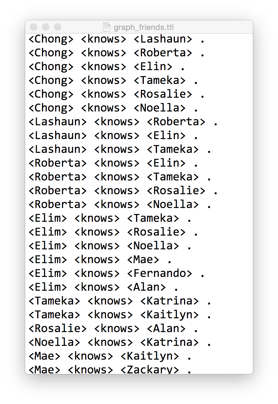
Here is what a sample looks like (graph_friends.ttl) that we can load into SPARQLverse with the above command:
Sample friends graph in Turtle format for loading into SPARQLverse graph analytic engine.
It includes 57 specific relationships. The first part of the triple is the Subject, the second is the Predicate/relationship made to the third part, the Object. If you look through the data you’ll see that all the Objects are also defined as Subjects that have other relationships.
Understand the basics here and you’ve got Triples almost mastered.
Note: This is an overly simplistic example, but not totally unrealistic. We don’t use any URIs but we are allowed to fake them here by simply putting angle brackets around them. In a linked data environment you’d establish your own namespaces and likely link to external SPARQL endpoints or resources with http:// prefixes. Now that starts to make your eyes crossed.
Quick Visualisation
As an aside, pull the sample data into Gephi to visualise it and you’ll see the intertwining relationships are not intuitive and would be a challenge to understand using a SQL relational approach.
Graph density represents how interconnected all entities in the graph are. They are a sort of ratio between the total number of connected nodes over maximum number of potential edges. The value ranges from 0 to 1 – with 0 being a total disconnected graph (not sure if that is technically a graph) with no interconnections between nodes. And 1 representing a high density graph where all nodes connect to all other nodes.
Here we use a SPARQL query to compute graph density, using the sample dataset above, run from the command line. (Note that I use “?knows” as a predicate when I really want to use “<knows>” but wordpress is not displaying that properly):
$ isbx -c "
 SELECT (?nrEdges/(?nrNodes *(?nrNodes - 1.0)) AS ?graphDensity)
 FROM <graphname>
 WHERE {
  { SELECT (COUNT (*) AS ?nrEdges) (COUNT (DISTINCT ?person) AS ?nrNodes)
    WHERE { ?person ?knows ?anotherPerson . }
   }
 }
"
graphDensity
-------------
0.150000
I changed the example “tips” query to use a different graph name (mygraph) and a different relationship name (knows). The sub-query in the WHERE clause first counts up the number of edges/relationships and counts the distinct number of nodes as well. Then the primary query compares that number of edges to nodes.
Let’s break that down into its detail…
Compute the number of unique nodes in the graph
$ isbx -c "SELECT (count (distinct ?person) as ?nrNodes)
> FROM <graphname> WHERE { ?person ?knows ?anotherPerson .}"
nrNodes
--------
20
This tells us that there are 20 people as Subjects in the graph. Therefore, a maximum number of edges between all people would be 20² (we’ll use only 20×19 as a person might not link to themselves in this example).
Compute the number of edges in the graph
$ isbx -c "SELECT (count (*) as ?nrEdges)
FROM <graphname> WHERE { ?person ?knows ?anotherPerson .}"
nrEdges
--------
57
Total edges is 57. Do the quick math and see that the ratio is then:
57 / (20 x 19)
= 57 / 380
= 0.149...
Challenge: Inverse Relationships in SPARQL
In some graphs you may not have all the people in the Object position (third part of triple) initialised as Subjects – and their names only show up when someone else defines a relationship to them.
In that case, your density from this query will under-report. I leave it as an exercise to the reader to figure out how to use SPARQL to do an optional inverse relationship in the sub-query WHERE clause. Ping me if you want some tips on that.
Future Post
In a future post I’ll walk through some of other graph query examples using SPARQL such as:
SPARQLverse is part of the Actian Analytics Platform – providing Big Data solutions that are hyper performance with ultimate scalability. Our SQL in Hadoop is the fastest available and runs truly in Hadoop 100%.
Need to “Perform Big Data Analytics at Massive Scale?” The Actian Analytics Platform includes the Matrix high performance analytics database (formerly known as Paraccel).
I’ve seen some people asking online for what JDBC URL syntax is. If you are using the JDBC driver be sure to read the README which gives the details:
The driver recognises JDBC URLs of the form: jdbc:paraccel:database
jdbc:paraccel://host/database
jdbc:paraccel://host:port/database

Also, you can supply both username and passwords as arguments, by appending them to the URL. For example:
jdbc:paraccel:database?user=me
jdbc:paraccel:database?user=me&password=mypass

Notes:
1) If you are connecting to localhost or 127.0.0.1, you can leave the host out of the URL; that is, jdbc:paraccel://localhost/mydb can be replaced with jdbc:paraccel:mydb
2) The port defaults to 5439 if it is not specified.