This blog post I wrote for Locate Press helps set the stage for those new to the scene of mapping, geography, spatial data, and application development.
Tag: geospatial
Make Stellar/Star Data Maps In GIS
I have a latent interest in stargazing but haven’t done much about it for a long time until the past weekend when I had a bit of time and wondered if I could create a star map using QGIS. I found a couple tutorials and stackexchange questions that referenced David Nash’s HYG Database from www.Astronexus.com. Some of the tutorials showed equations for computing latitude and longitude from the star position values – ascension, declination specifically. However, I found that there is already an X and Y column in the latest version of the dataset which makes it easy to map, here’s how.
Download the Star Location Data
From the HYG Database page, grab the HYG version 3.0 dataset:
- HYG 3.0: Database containing all stars in Hipparcos, Yale Bright Star, and Gliese catalogs (almost 120,000 stars, 14 MB)
The resulting 34MB CSV file contains about 20 columns and 119,615 rows.
Import CSV File into QGIS
- Launch QGIS (I’m using 2.10.1-Pisa)
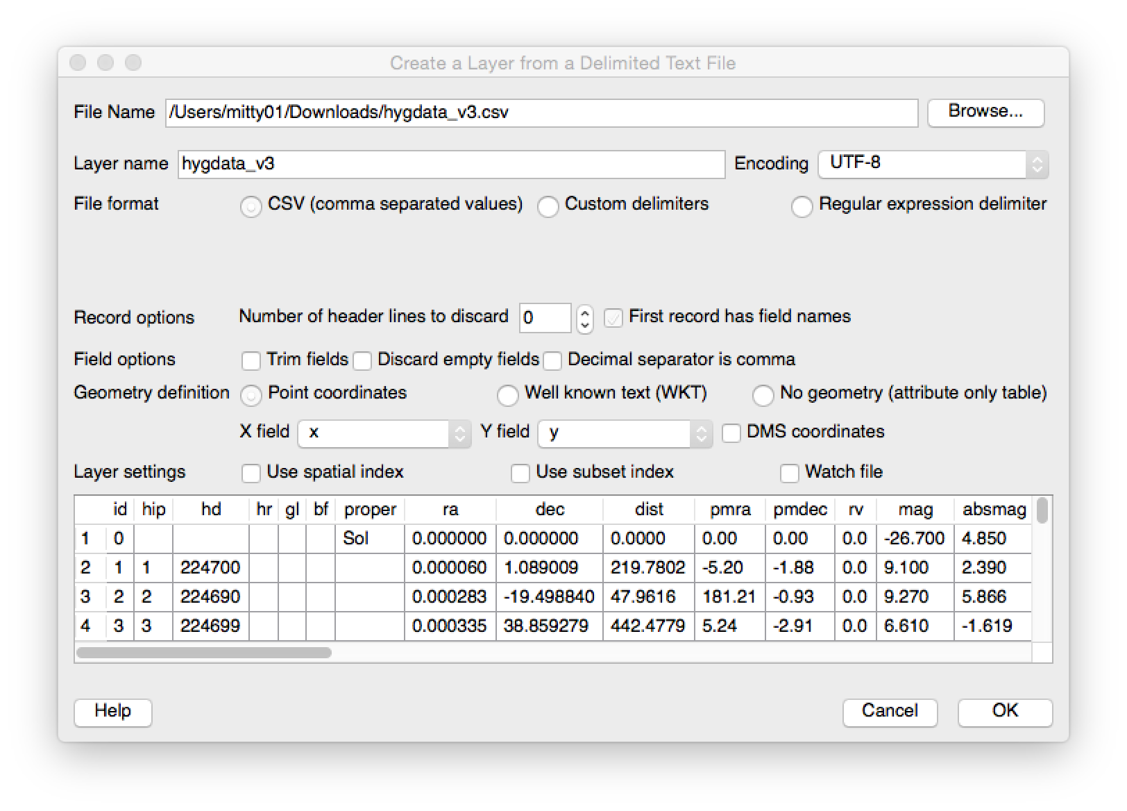
- Select Layer -> Add Layer -> Add Delimited Text Layer
- Browse to the file location, select File Format radio button as CSV and the rest should take care of itself
Tweak the Map
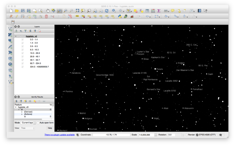
If you use a typical WGS84 projection you’ll get a ton of points oriented in a circle. I took a few minutes to zoom into a meaningful scale (for me it was around 1:5M), change the background colour and then use the LUM attribute to change the relative size of the stars. I also changed the colours to be shades of white. Here is what I was able to produce. It’s not all that meaningful to me but I know that when I need to dig into the data further it will be available!
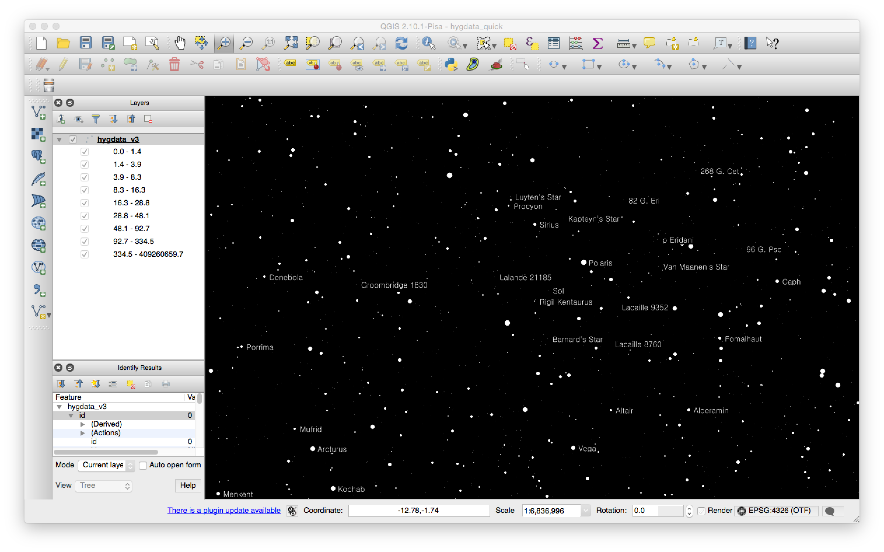
I’ve attached my project file here so you can get started quickly.
I’d love to hear what you would use this kind of data for and if you have any tips for making it more useful or better rendered.
Day 1 – Building a 3D Game using Geo Data (Hobby project)
We are a team of three guys (so far) with a design idea for a simple yet challenging racing/strategy game based on real-world geospatial data coupled with a 3D gaming engine. Tonight we started building it together in Unity after downloading a bunch of public geospatial datasets. Here’s a summary of what we’ve done and some basic screenshots. The goal is to make progress every couple days to show we is possible with a little work and a combination of creative, technical and group management skillsets.
First Images
Starting with Geography
The landscape of our 3D game is built using real world geographic information – aka geospatial data. We wanted this so that we could build games around real locales and market the game to local users. One side benefit is the players will learn a little about Canadian geography!
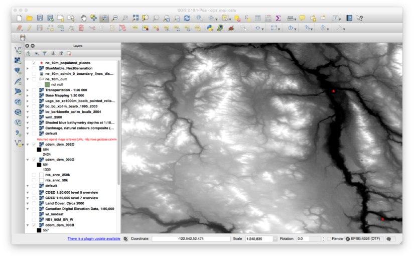
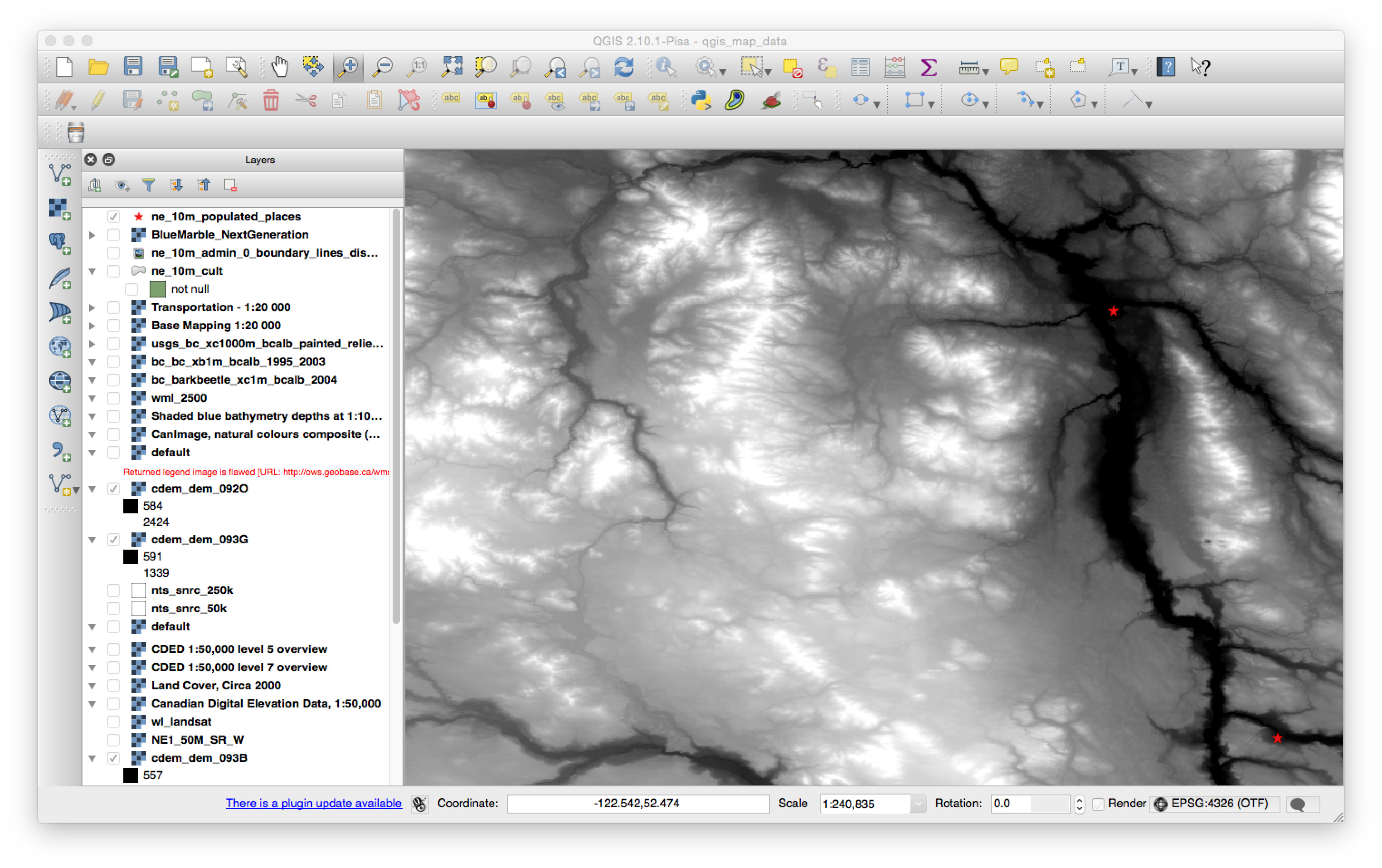
We’ve got a great collection of geo data for all of Canada available through the government Geogratis website. After we’ve decided what map tile numbers we needed, we grab the CDED data which is a TIFF elevation image file with geographic coordinates included.
We also found a BC provincial shaded relief map layer that was pretty nice as a starter. As both these data files are geolocated we can load the data into GIS (geographic information system) software from QGIS.org and combine it with any other data we have for the region. In our case we have a “populated places” point file from naturalearthdata.org that we show as stars on top of the shaded relief map.
Then we export the elevation data and the relief data (including the stars) into two files for Unity to ingest. The result is one PNG that is going to be our texture and the other will be the heightmap for the terrain.
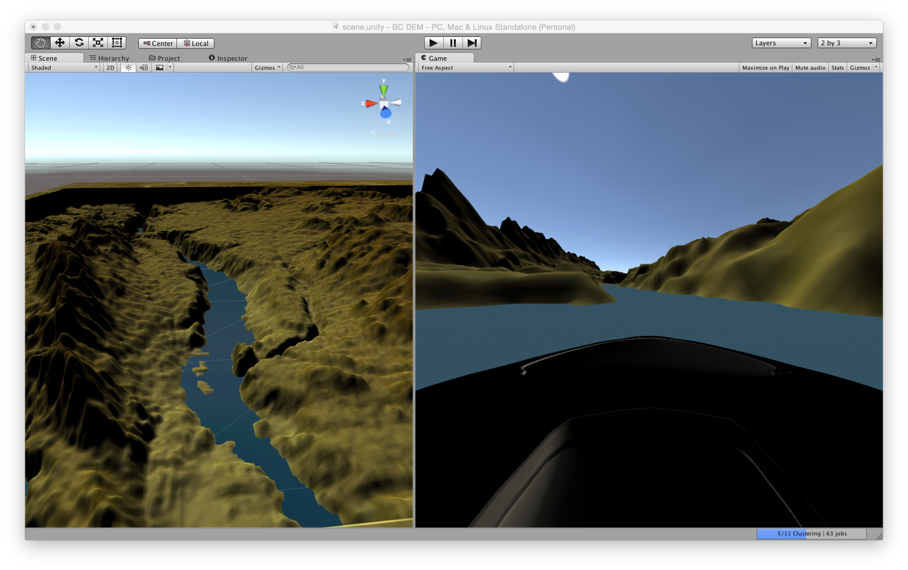
Loading into Unity
We created a terrain object with some pretty huge dimensions and height. There are mountains in the region we are working with, so it’s pretty cool to see. We apply the heightmap using a commonly used Unity script (I’ll have to put the link here when I remember where I got it!).
Then we add the shade relief map as a texture to the terrain et voila! We threw in a plane of basic water and raised it to the level where it filled the main river valleys. As our game is going to first start as a river racing game, we want to start with water from the very beginning.
We added a car, parented it to the camera and were racing down our waterways within 2 hours of starting. We spent a lot of time adjusting sizes of terrains and texture so we could try to match real-world scale. There are some further ideas we are going to try to optimise this as well as nail down a workflow for easily ingesting new geodata for other regions (as we had to manually export and adjust things in the GIS).
Reposted from our Indiedb blog, hence writing for a slightly non-geo audience: http://www.indiedb.com/members/1tylermitchell/blogs/edit/1mitchellco-day-1-cross-country-river-run-race-game
Generate terrain with flowing water from DEM in Unity
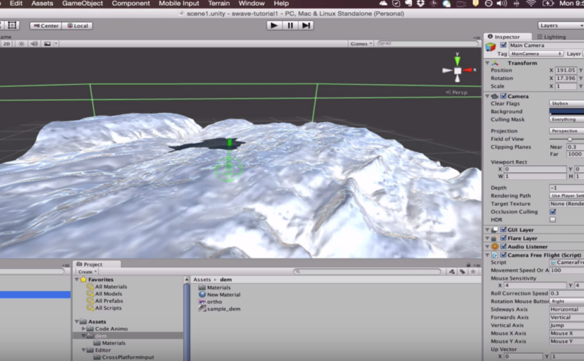
Just a quick video follow up based on a reader asking how I did what I did in my previous post with Unity (http://unity3d.com) game engine.
Using Surface Wave asset and built-in Unity Terrain generator, plus a script for taking DEMs and creating Terrains easily. I’m really new at this by the way, but have a brilliant teacher showing me this stuff in my spare time 🙂
High speed water flow simulation on a DEM
I’m helping some friends who are working on a project to visualise a whole whack of GIS data in Unity (Unity3D.com) game engine. It looks like we’ll end up working on a GIS -> Unity workflow for generating terrains from DEMs and texture maps from orthophotos. To top it off they’ve already got a landcover classification app running that takes landcover raster classes and creates 3D objects (grass, trees, water) in the model. (Don’t worry, I won’t tease you by mentioning their voxel based subsurface soil model interaction). It’s still early but really encouraging so far.
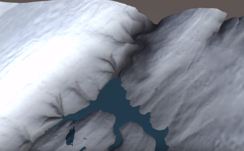
Next up is to simulate water flow in the environment and it was slim pickings for options for doing this. Then they found the Unity asset called Surface Waves (US$80) – it does the water flow work we wanted but much more. I just posted a really short test video to see how it worked – with both an auto generated water source and a manual placement water source, like a paint brush, that allows you to see how things will flow. It is amazingly performant on a notebook.
Be sure to check out Surface Waves’ demo video – it frees you from trying to emulate the look of water movement through shader trickery to actually simulating water flow over and around objects. Things that used to take a sophisticated GIS quite a while to compute actually, the last time I tried anyway 🙂
More to come as we play around with it, but I put it out there in case other spatially oriented folks might be interested as well in the GIS -> Unity workflow challenges being worked through. If so, I’ll do more video highlighting the work that’s underway.
Geospatial Power Tools Reviews [Book]
Thinking of buying my latest book? We’ve finally got a few reviews on Amazon that might help you decide. See my other post for more about the book. Buy the PDF on Locate Press.com.
Reader Reviews
January 24, 2015 By Leo Hsu
“The GDAL Toolkit is chuckful of ETL commandline tools for working with 100s of spatial (and not so spatial data sources). Sadly the GDAL website only provides the basic API command switches with very few examples to get a user going with. I was really excited when this book was announced and purchased as soon as it came out. This book makes a great reference manual for using GDAL/OGR suite of command line utilities.Several chapters are devoted to each commandline tool, explaining what its for, the switches it has, and several examples of how to use each one. You’ll learn how to work with both vector/(basic data no vector) data sources and how to convert from one vector format to another. You’ll also learn how to work with raster data and how to transform from one raster data source to another as well as various operations you can perform on these.”
Converting Decimal Degree Coordinates
Converting Decimal Degree Coordinates to/from DMS Degrees Minutes Seconds
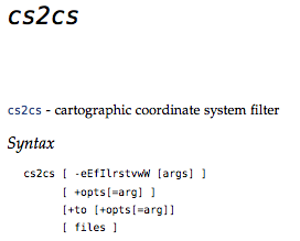
If you have files or apps that have to filter or convert coordinates – then the cs2cs command is for you. It comes with most distributions of the GDAL/OGR (gdal.org) toolset. Here is one popular example for converting between degrees minutes and seconds (DMS) and decimal degrees (DD).
 The following is an excerpt from the book: Geospatial Power Tools – Open Source GDAL/OGR Command Line Tools by me, Tyler Mitchell. The book is a comprehensive manual as well as a guide to typical data processing workflows, such as the following short sample…
Input coordinates can come from the command line or an external file. Assuming a file containing DMS (degree, minute, seconds) style, looks like:
124d10'20"W 52d14'22"N

122d20'05"W 54d12'00"N
Use the cs2cs command, specifying how the print format will be returned, using the -f option. In this case -f “%.6f”
is explicitly requesting a decimal degree number with 6 decimals:
cs2cs -f "%.6f" +proj=latlong +datum=WGS84 input.txt
Example Converting DMS to/from DD
This will return the results, notice no 3D/Z value was provided, so none is returned:
-124.172222 52.239444 0.000000

-122.334722 54.200000 0.000000
To do the inverse, remove the formatting option and provide a list of values in decimal degree (DD):
cs2cs +proj=latlong +datum=WGS84 inputdms.txt

124d10'19.999"W 52d14'21.998"N 0.000

122d20'4.999"W 54d12'N 0.000
Geospatial Power Tools is 350+ pages long – 100 of those pages cover these kinds of workflow topic examples. Each copy includes a complete (edited!) set of the GDAL/OGR command line documentation as well as the following topics/examples:
Workflow Table of Contents
- Report Raster Information – gdalinfo
- Web Services – Retrieving Rasters (WMS)
- Report Vector Information – ogrinfo
- Web Services – Retrieving Vectors (WFS)
- Translate Rasters – gdal_translate
- Translate Vectors – ogr2ogr
- Transform Rasters – gdalwarp
- Create Raster Overviews – gdaladdo
- Create Tile Map Structure – gdal2tiles
- MapServer Raster Tileindex – gdaltindex
- MapServer Vector Tileindex – ogrtindex
- Virtual Raster Format – gdalbuildvrt
- Virtual Vector Format – ogr2vrt
- Raster Mosaics – gdal_merge

Create Tile Map Structure – gdal2tiles command
Tiles in a Tile Map Server (TMS) context are basically raster map data that’s broken into tiny pre-rendered tiles for maximum web client loading efficiency. GDAL, with Python, can chop up your input raster into the folder/file name and numbering structures that TMS compliant clients expect.
This is an excerpt from the book: Geospatial Power Tools – Open Source GDAL/OGR Command Line Tools by me, Tyler Mitchell. The book is a comprehensive manual as well as a guide to typical data processing workflows, such as the following short sample…
The bonus with this utility is that it also creates a basic web mapping application that you can start using right away.
The script is designed to use georeferenced rasters, however, any raster should also work with the right options. The (georeferenced) Natural Earth raster dataset is used in the first examples, with a non-georeferenced raster at the end.
There are many options to tweak the output and setup of the map services; see the complete gdal2tiles chapter for more information.
Minimal TMS Generation
At the bare minimum an input file is needed:
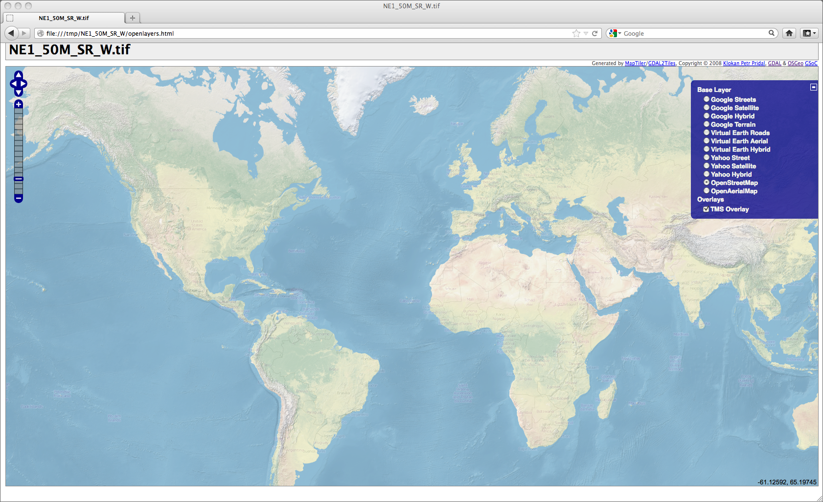
gdal2tiles.py NE1_50M_SR_W.tif
Generating Base Tiles:
0...10...20...30...40...50...60...70...80...90...100 - done.
Generating Overview Tiles:
0...10...20...30...40...50...60...70...80...90...100 - done.
The output created is the same name as the input file, and include an array of sub-folders and sample web pages:
NE1_50M_SR_W
NE1_50M_SR_W/0
NE1_50M_SR_W/0/0
NE1_50M_SR_W/0/0/0.png
NE1_50M_SR_W/1
...
NE1_50M_SR_W/4/9/7.png
NE1_50M_SR_W/4/9/8.png
NE1_50M_SR_W/4/9/9.png
NE1_50M_SR_W/googlemaps.html
NE1_50M_SR_W/openlayers.html
NE1_50M_SR_W/tilemapresource.xml
Open the openlayers.html file in a web browser to see the results.
| The default map loads a Google Maps layer, it will complain that you do not have an appropriate API key setup in the file, ignore it and switch to the OpenStreetMap layer in the right hand layer listing. |
The resulting map should show your nicely coloured world map image from the Natural Earth dataset. The TMS Overlay option will show in the layer listing, so you can toggle it on/off to see that it truly is loading. Figure 5.2 (above) shows the result of our gdal2tiles command.
Geospatial Power Tools is 350+ pages long – 100 of those pages cover these kinds of workflow topic examples. Each copy includes a complete (edited!) set of the GDAL/OGR command line documentation as well as the following topics/examples:
Workflow Table of Contents
- Report Raster Information – gdalinfo 23
- Web Services – Retrieving Rasters (WMS) 29
- Report Vector Information – ogrinfo 35
- Web Services – Retrieving Vectors (WFS) 45
- Translate Rasters – gdal_translate 49
- Translate Vectors – ogr2ogr 63
- Transform Rasters – gdalwarp 71
- Create Raster Overviews – gdaladdo 75
- Create Tile Map Structure – gdal2tiles 79
- MapServer Raster Tileindex – gdaltindex 85
- MapServer Vector Tileindex – ogrtindex 89
- Virtual Raster Format – gdalbuildvrt 93
- Virtual Vector Format – ogr2vrt 97
- Raster Mosaics – gdal_merge 107
Create a Union VRT from a folder of Vector files
The following is an excerpt from the book: Geospatial Power Tools – Open Source GDAL/OGR Command Line Tools by me, Tyler Mitchell. The book is a comprehensive manual as well as a guide to typical data processing workflows, such as the following short sample…
The real power of VRT files comes into play when you want create virtual representations of features as well. In this case, you can virtually tile together many individual layers as one. At the present time you cannot do this with a single command line but it only takes adding two simple lines to the VRT XML file to make it start working.
Here we want to create a virtual vector layer from all the files containing lines in the ne/10m_cultural folder.
First, to keep it simple, create a folder and copy in only the files we are interested in:
mkdir ne/all_lines
cp ne/10m_cultural/*lines* ne/all_lines
Then we can create our VRT file using ogr2vrt as shown in the previous example:
python ogr2vrt.py -relative ne/all_lines all_lines.vrt
If added to QGIS at this point, it will merely present a list of four layers to select to load. This is not what we want.
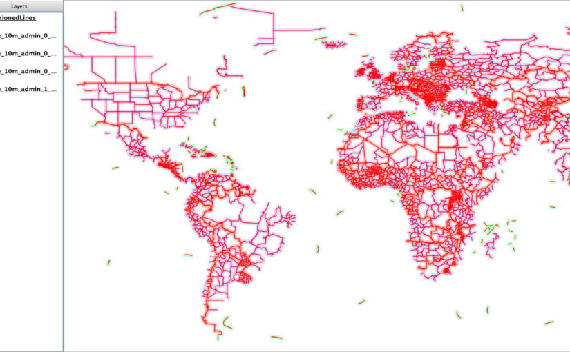
So next we edit the resulting all_lines.vrt file and add a line that tells GDAL/OGR that the contents are to be presented as a unioned layer with a given name (i.e. “UnionedLines”).
The added line is the second one below, along with the closing line second from the end:
<OGRVRTDataSource>
 <OGRVRTUnionLayer name="UnionedLines">
  <OGRVRTLayer name="ne_10m_admin_0_boundary_lines_disputed_areas">
   <SrcDataSource relativeToVRT="1" shared="1">
   ...
   <Field name="note" type="String" src="note" width="200"/>
  </OGRVRTLayer>
 </OGRVRTUnionLayer>
</OGRVRTDataSource>
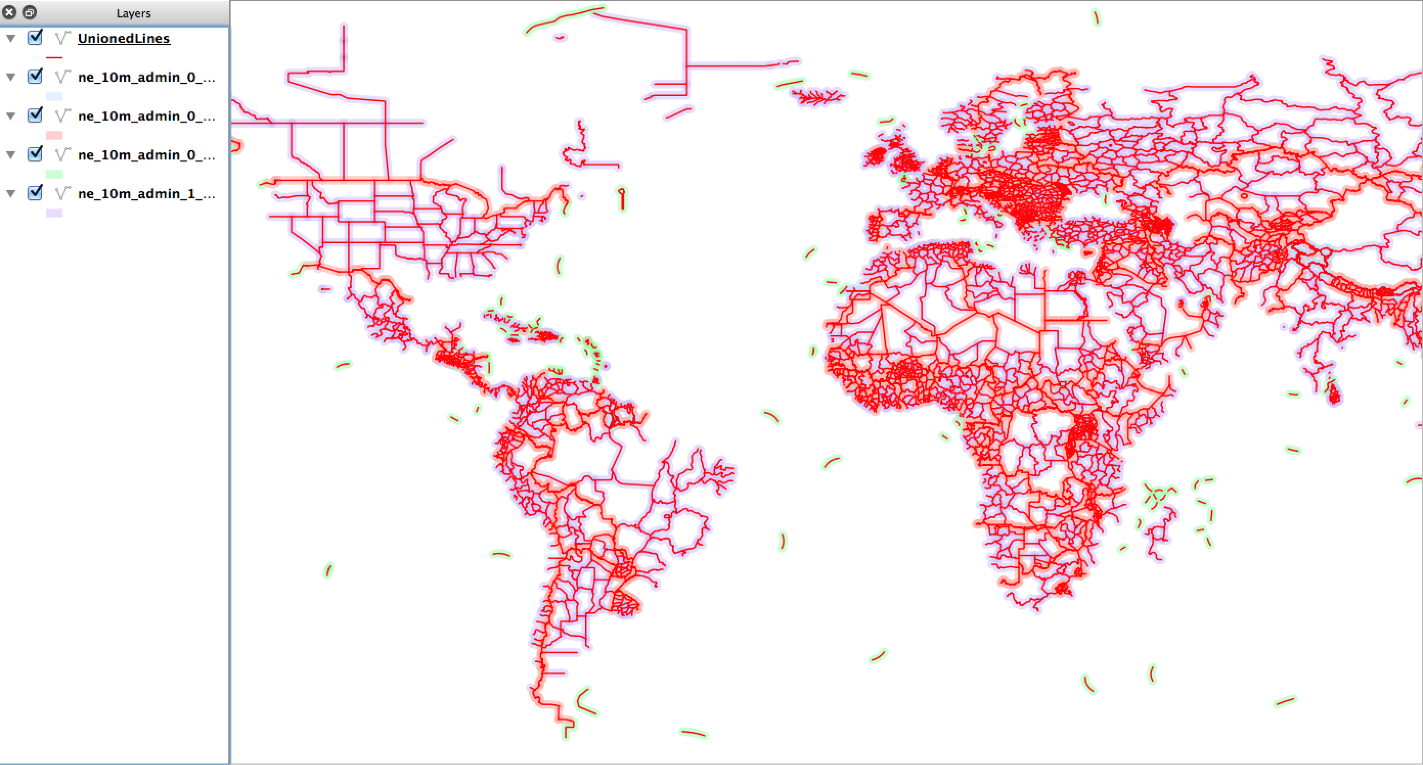
Now loading it into QGIS automatically loads it as a single layer but, behind the scenes, it is a virtual representation of all four source layers.
On the map in Figure 5.8 the unionedLines layer is drawn on top using red lines, whereas all the source files (that I manually loaded) are shown with a light shading. This shows that the new virtual layer covers all the source layer features.
Geospatial Power Tools is 350 pages long – 100 of those pages cover these kinds of workflow topic examples. Each copy includes a complete (edited!) set of the GDAL/OGR command line documentation as well as the following topics/examples:
Workflow Table of Contents
- Report Raster Information – gdalinfo 23
- Web Services – Retrieving Rasters (WMS) 29
- Report Vector Information – ogrinfo 35
- Web Services – Retrieving Vectors (WFS) 45
- Translate Rasters – gdal_translate 49
- Translate Vectors – ogr2ogr 63
- Transform Rasters – gdalwarp 71
- Create Raster Overviews – gdaladdo 75
- Create Tile Map Structure – gdal2tiles 79
- MapServer Raster Tileindex – gdaltindex 85
- MapServer Vector Tileindex – ogrtindex 89
- Virtual Raster Format – gdalbuildvrt 93
- Virtual Vector Format – ogr2vrt 97
- Raster Mosaics – gdal_merge 107
Query Vector Data Using a WHERE Clause – ogrinfo
The following is an excerpt from the book: Geospatial Power Tools – Open Source GDAL/OGR Command Line Tools by Tyler Mitchell. The book is a comprehensive manual as well as a guide to typical data processing workflows, such as the following short sample…
Use SQL Query Syntax with ogrinfo
Use a SQL-style -where clause option to return only the features that meet the expression. In this case, only return the populated places features that meet the criteria of having NAME = ’Shanghai’:
$ ogrinfo 10m_cultural ne_10m_populated_places -where "NAME = 'Shanghai'"

...
Feature Count: 1 Extent: (-179.589979, -89.982894) - (179.383304, 82.483323)
...
OGRFeature(ne_10m_populated_places):6282
 SCALERANK (Integer) = 1
 NATSCALE (Integer) = 300
 LABELRANK (Integer) = 1
 FEATURECLA (String) = Admin-1 capital
 NAME (String) = Shanghai
...
 CITYALT (String) = (null)
 popDiff (Integer) = 1
 popPerc (Real) = 1.00000000000
 ls_gross (Integer) = 0
 POINT (121.434558819820154 31.218398311228327)
Building on the above, you can also query across all available layers, using the -al option and removing the specific layer name. Keep the same -where syntax and it will try to use it on each layer. In cases where a layer does not have the specific attribute, it will tell you, but will continue to process the other layers:
ERROR 1: 'NAME' not recognised as an available field.
NOTE: More recent versions of ogrinfo appear to not support this and will likely give FAILURE messages instead.
Geospatial Power Tools is 350 pages long – 100 of those pages cover these kinds of workflow topic examples. Each copy includes a complete (edited!) set of the GDAL/OGR command line documentation as well as the following topics/examples:
Workflow Table of Contents
- Report Raster Information – gdalinfo 23
- Web Services – Retrieving Rasters (WMS) 29
- Report Vector Information – ogrinfo 35
- Web Services – Retrieving Vectors (WFS) 45
- Translate Rasters – gdal_translate 49
- Translate Vectors – ogr2ogr 63
- Transform Rasters – gdalwarp 71
- Create Raster Overviews – gdaladdo 75
- Create Tile Map Structure – gdal2tiles 79
- MapServer Raster Tileindex – gdaltindex 85
- MapServer Vector Tileindex – ogrtindex 89
- Virtual Raster Format – gdalbuildvrt 93
- Virtual Vector Format – ogr2vrt 97
- Raster Mosaics – gdal_merge 107